Barcodes and diversity - Fastq read analysis for 16S rRNA metabarcoding using the R package DADA2

Professor Patrick Biggs

Purpose
Introduction
Lecture Overview
Conventions used for this RStudio practical
Accessing the resources needed
Theoretical overview
Exercise 1: Getting everything ready
Exercise 2: Collecting our data
Exercise 3: Examining the quality profiles of forward and reverse reads
Exercise 4: Performing filtering and trimming
Exercise 5: Dereplication
Exercise 6: Investigation of the error rates
Exercise 7: Sample inference
Exercise 8: Merging the paired reads
Exercise 9: Constructing the sequence table and removing chimaeras
Exercise 10: Checking our progress
Exercise 11: Assigning taxonomy
Exercise 12: Evaluating the accuracy
Exercise 13: Working with fasta files to generate a sequence logo
Portfolio analysis
Assessment
Contact

Purpose

To learn how to perform an analysis of 16S rRNA sequencing data from raw sequencing data to preliminary visualisation and taxonomic classification.

Introduction

Microbial diversity has been revolutionised by the rapid advances in sequencing technology, given us new insights into the role of the microbial world in all environments on Earth. Sequencing of metagenomes (all the DNA in a given sample etc) or of specific markers (metabarcodes e.g. 16S rRNA amplicons) have been crucial in this regard. Knowing what is there, and what it is potentially doing are two of the main research areas of interest. How we then analyse the data, visualise and interpret the results is thus of importance.

Week 8 focusses on introducing ideas around the analysis of microbial diversity - for bacteria - within the 16S rRNA amplicon, and performing a typical workflow analysis on such sequences in R using a piece of software called DADA2. These ideas will be developed further in the next two weeks (weeks 9 and 10) of this module.

An outline of the labs during Weeks 8 and 10 is below.

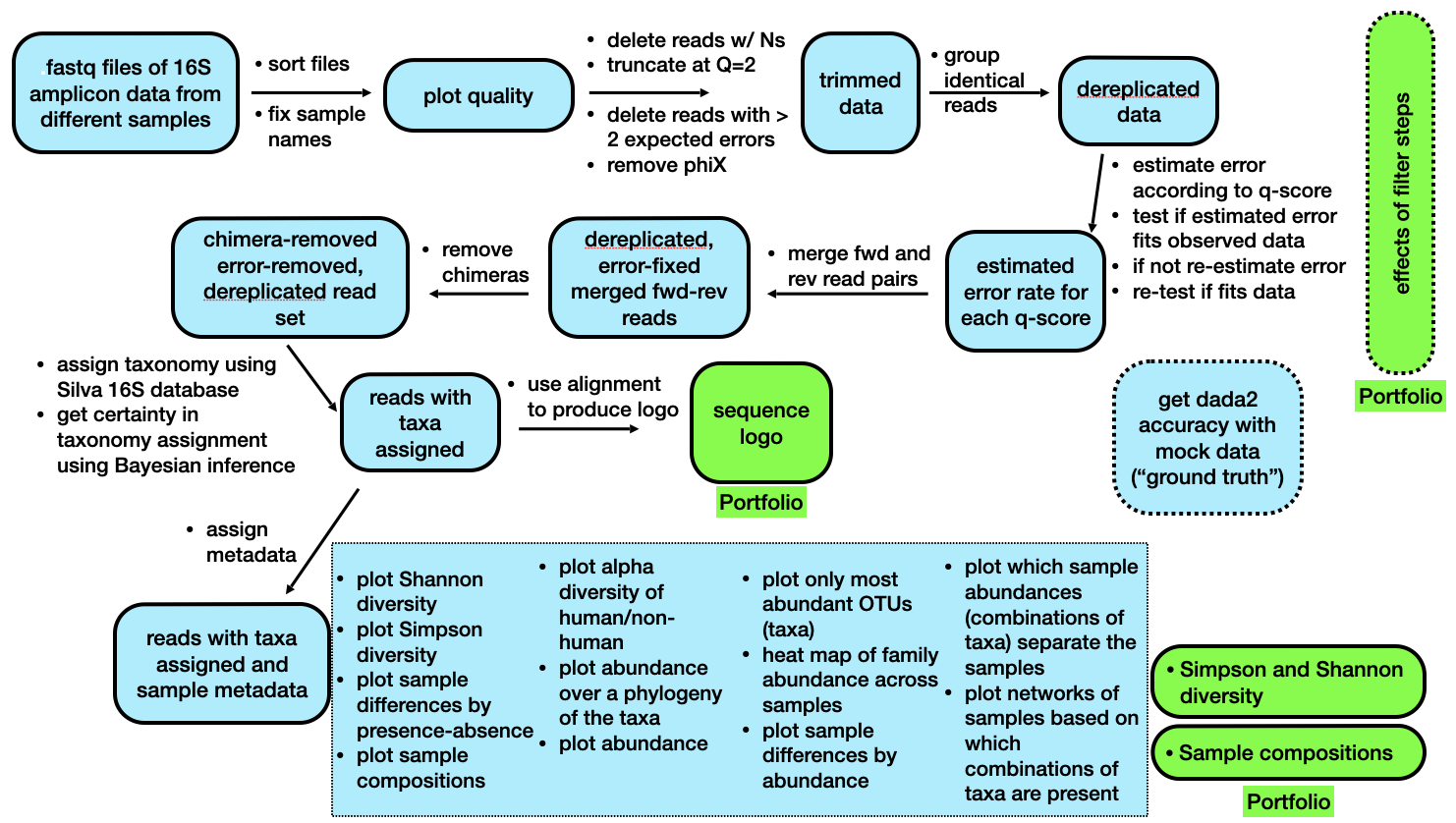
Brief outline of the steps we will be following in Week 8 (today) and Week 10.

Lecture Overview

The lecture introduced the motivation for doing these kinds of studies, and described the very important conceptual difference between metabarcoding and metagenomics. Next an overview of metabarcoding was discussed as was the 16S rRNA amplicon, and some initial ideas about how we work with sequence diversity to make OTUs (operational taxonomic units).

We then swtiched tack to looking at software - from a historical point of view - with QIIME, mothur and Usearch being mentioned before turning or focus to DADA2 within the R environment. Finally some challenges were mentioned, which is a theme further developed in the tutorial.

So, now on to the practical…

First thing, you have an electronic copy of this practical – which you will see via the Stream and this site – please don’t copy and paste in the practical today! Why? Typing these commands is part of the hard wiring required to make them stick! By typing commands it gives you another opportunity to think about the command before you execute it and typing is more likely to trigger a big red flag in dangerous situations! So, think twice, type once, we will discuss this more next week.

Conventions used for this RStudio practical

As a reminder, in what follows, we shall use the following typographical conventions for working with R:

Characters written in this programming style are commands to be typed into the computer as they stand.
Characters written in this programming style are objects and file names.
Characters written after something like ### indicate comments within the code that will help you. They do not run code.
Characters written in without > at the start of the line (e.g. lines starting with “[1]”) indicate responses back from the R console inside RStudio that will help you too.
Words inserted within square brackets [Enter] indicate keys to be pressed.

So, for example,

 > x <- c(1, 5, 7, 14) [Enter]

means "at the R console prompt >, type the code as written to make a vector x made up of the values 1, 5, 7 and 14, then press the key marked Enter".

Don't forget to press the [Enter] key: commands are not sent to the R console until this is done. There will not be [Enter] at the end of any of the lines of code in this practical, it is taken that this is to be typed at the end of the line unless otherwise stated. It is also assumed that the first > is the R console prompt.

Accessing the resources needed

Computing

General

We will be working within web browsers, and Firefox and Chrome are installed on the machines, or Safari if you are an Apple user. We will then login to RStudio Cloud using your personalised account. If you would like to use your own laptop in the labs on either campus, please feel free to do so.

Manawatu (iMacs)

The machines we are using for the course are Apple iMacs. Please use your normal Massey username and password to login to these machines. Please remember to ignore (i.e. cancel) the dialogue box about the network when you log in.

Albany (PCs)

The machines are Windows PC’s so logging into them should be the same as any other Massey Windows PC.

outside Massey

Most likely this is your own machine, so this should not be an issue.

Our work today

Just as we did for the Bootcamp module, you have been provided with a link to create a new RStudio workspace in your account. Please go ahead and do this if you have not already done so. We are using different packages in R for this Module - some of which have large numbers of dependencies (I have loaded them for you already) - so I strongly suggest starting this new Module with this new workspace. Also, the resources for this Module will only be available via this project (I will be posting the files on Stream as well as a backup).

Theoretical overview

The DADA2 paper¹ by Callahan et al. has an associated GitHub page² and a great tutorial page. We are going to use a set of 20 samples that are used in the tutorial, and are provided for you within the MiSeq_SOP folder. There are other files in there, but more on those later. So, most of the below comes from the tutorial and the DADA2 vignette inside R and is acknowledged as such.

The investigation of environmental microbial communities and microbiomes has been driven in significant part by the recent widespread adoption of amplicon sequencing. In amplicon sequencing a particular genetic locus is amplified from DNA extracted from the community of interest, and then sequenced on a next-generation sequencing platform. This technique removes the need to culture microbes in order to detect their presence, and cost-effectively provides a deep census of a microbial community.

However, the process of amplicon sequencing introduces errors into the DNA sequences being analysed, and these errors severely complicate the interpretation of the results. DADA2 implements a novel algorithm that models the errors introduced during amplicon sequencing and uses that error model to infer the true sample composition. DADA2 takes the place of the ubiquitous “OTU-picking” step in amplicon sequencing workflows. As demonstrated in the paper and in further benchmarking, the DADA2 method provides both better sensitivity and specificity than OTU methods: DADA2 detects real biological variation missed by OTU methods while outputting fewer spurious sequences.

The starting point for the DADA2 pipeline is a set of demultiplexed Fastq files corresponding to the samples an amplicon sequencing study. That is, DADA2 expects there to be an individual Fastq file for each sample (or two Fastq files, one forward and one reverse, for each sample). Once demultiplexed Fastq files are in hand, the DADA2 pipeline proceeds as follows:

Filter and Trim: filterAndTrim()
Dereplicate: derepFastq()
Learn error rates: learnErrors()
Infer sample composition: dada()
Merge paired reads: mergePairs()
Make sequence table: makeSequenceTable()
Remove chimeras: isBimeraDenovo() or removeBimeraDenovo()
Assign taxonomy: assignTaxonomy()

The output of the DADA2 pipeline is a sample-by-sequence matrix – a so-called sequence table – with each entry corresponding to the number of times that inferred sample sequence was observed in that sample. This table is analogous to a common OTU table, except at higher resolution (exact sample sequences rather than 97% OTUs). We also assign taxonomies to the output sequences using a small reference database. In this practical we are working with a small set of Fastq reads from the 16S rRNA gene – one of the main taxonomic identifiers in prokaryotes.

What we are going to do today?

We start out with a set of Illumina-sequenced paired-end Fastq files that have been split (or “demultiplexed”) by sample and from which the barcodes/adapters have already been removed.
We will end up with an amplicon sequence variant (ASV) table, a higher-resolution analogue of the ubiquitous “OTU table”, which records the number of times each 16S rRNA sequence variant (SV) was observed in each sample.

Exercise 1: Getting everything ready

We will check we have all we need to do the analysis first. The commands below have been checked and should work fine. The below screenshot shows the folder structure within /cloud/project/ for the new Module.

Go to the MiSeq_SOP folder in the /cloud/project/ project within the “weeks8to10” project within the “MicrobialDiversity_2023” workspace and check that there are files there.

Check we have all our packages we need for the work, so typing into the console as you have done before:

### check on packages being there and their versions ###
> library(dada2)
> packageVersion("dada2")
[1] ‘1.28.0’

> library(ShortRead)
> packageVersion("ShortRead")
[1] ‘1.58.0’

> library(ggplot2)
> packageVersion("ggplot2")
[1] ‘3.4.2’

The next thing we want to do is to set a working path and then define a path variable to check it is all OK for the work we are going to do today.

### is our path OK?
> path <- ("/cloud/project/MiSeq_SOP/")
> path
[1] "/cloud/project/MiSeq_SOP/"

> fns <- list.files(path)
> fns
 [1] "F3D0_S188_L001_R1_001.fastq"   "F3D0_S188_L001_R2_001.fastq"   "F3D1_S189_L001_R1_001.fastq"  
 [4] "F3D1_S189_L001_R2_001.fastq"   "F3D141_S207_L001_R1_001.fastq" "F3D141_S207_L001_R2_001.fastq"

If you do not see this structure and output, please let a demonstrator know as soon as possible, as you will not be able to proceed any further in the practical without it.

Question 1: How many non-Fastq files are there in the directory?

____________________

Exercise 2: Collecting our data

First we read in the names of the Fastq files, and perform some string manipulation to get lists of the forward and reverse Fastq files in matched order. This is relatively straightforward, so we shall just go ahead and do this.

### extract out our fastq sequences
> fastqs <- fns[grepl(".fastq$", fns)]
> fastqs
[1] "F3D0_S188_L001_R1_001.fastq"   "F3D0_S188_L001_R2_001.fastq"   "F3D1_S189_L001_R1_001.fastq"  
[4] "F3D1_S189_L001_R2_001.fastq"   "F3D141_S207_L001_R1_001.fastq" "F3D141_S207_L001_R2_001.fastq"
[7] "F3D142_S208_L001_R1_001.fastq" "F3D142_S208_L001_R2_001.fastq" "F3D143_S209_L001_R1_001.fastq"

### sort them to ensure reads are in the same order
> fastqs <- sort(fastqs)

### make sub-lists for the forward and reverse reads
> fnFs <- fastqs[grepl("_R1", fastqs)] # Just the forward read files
> fnRs <- fastqs[grepl("_R2", fastqs)] # Just the reverse read files

### get the sample.names
> sample.names <- sapply(strsplit(fnFs, "_"), `[`, 1)

### Specify the full path to the fnFs and fnRs
> fnFs <- file.path(path, fnFs)
> fnRs <- file.path(path, fnRs)
> fnFs
 [1] "/cloud/project/MiSeq_SOP//F3D0_S188_L001_R1_001.fastq"  
 [2] "/cloud/project/MiSeq_SOP//F3D1_S189_L001_R1_001.fastq"  
 [3] "/cloud/project/MiSeq_SOP//F3D141_S207_L001_R1_001.fastq"
> fnRs
 [1] "/cloud/project/MiSeq_SOP//F3D0_S188_L001_R2_001.fastq"  
 [2] "/cloud/project/MiSeq_SOP//F3D1_S189_L001_R2_001.fastq"  
 [3] "/cloud/project/MiSeq_SOP//F3D141_S207_L001_R2_001.fastq"

Question 2: How many Fastq files are there in the directory?

____________________

Exercise 3: Examining the quality profiles of forward and reverse reads

It is important to look at your data. We start by visualizing the quality profiles along the sequencing reads.

### Visualize the quality profile of the forward reads
> plotQualityProfile(fnFs[[1]])
> plotQualityProfile(fnFs[[12]])
> plotQualityProfile(fnRs[[1]])
> plotQualityProfile(fnRs[[12]])

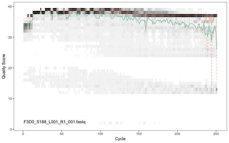
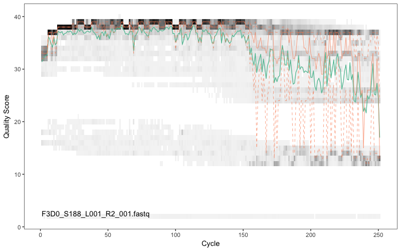
Here we have randomly picked sample 1 and sample 12. We are plotting the Phred quality scores for the Fastq reads for this sample (y-axis) against the sequencing cycle (x-axis). Clearly, we want our data to be as high quality as possible. The green line shows the median quality score at each position, and the orange lines shows the quartiles of the quality score distribution. The red line shows the scaled proportion of reads that extend to at least that position (this is more useful for other sequencing technologies, as Illumina reads are typically all the same length, hence the flat red line). Typical example plots look like the overleaf for the forward and reverse reads respectively for one of the samples:

Question 3: What do you think about the quality of read 1 (R1; forward) compared to read 2 (R2; reverse)?

____________________

The forward reads are of good quality. It would generally be advised that trimming the last few nucleotides is a good idea to avoid less well-controlled errors that can arise there. There is no suggestion from these quality profiles that any additional trimming is needed, so we will truncate the forward reads at position 240 (trimming the last 10 nucleotides). As is mostly the case, the reverse reads are of significantly worse quality, especially at the end, which is common in Illumina paired-end sequencing. This isn’t too worrisome, DADA2 incorporates quality information into its error model which makes the algorithm is robust to lower quality sequence, but trimming as the average qualities crash is still a good idea. We will truncate at position 160 where the quality distribution crashes.

Exercise 4: Performing filtering and trimming

Now that we know what our quality is like, we need to perform some filtering and trimming on the data. For this kind of work, having more – but poorer quality data – can have major deleterious consequences on data analysis.

As in the DADA2 tutorial, we will use standard filtering parameters: maxN=0 (DADA2 requires no Ns), truncQ=2 and maxEE=2. The maxEE parameter sets the maximum number of “expected errors” allowed in a read, which is a better filter than simply averaging quality scores. We use filterAndTrim() to jointly filter the forward and reverse reads.

### Make directory and filenames for the filtered fastqs
> filt_path <- file.path(path, "filtered")
> if(!file_test("-d", filt_path)) dir.create(filt_path)
> filt_path
[1] "/cloud/project/MiSeq_SOP//filtered"

### make list of filtered names for later
> filtFs <- file.path(filt_path, paste0(sample.names, "_F_filt.fastq.gz"))
> filtRs <- file.path(filt_path, paste0(sample.names, "_R_filt.fastq.gz"))

Question 4: The second line in the above R code is a complicated one – if(!file_test("-d", filt_path)) dir.create(filt_path) – can you work out what it might be doing (if you cannot, do not worry, this is a tricky one)?

____________________

Now to perform the actual filtering and trimming on our samples and place the results in an object called trim_data. Due to our RStudio Cloud setup this year, we have to run the code in a slightly different way. This is due to resources we are allowed in the cloud environment. These lines of code might take a couple of minutes or so to run.

### Perform the trimming and filtering
### Adapted for 2022
### You will not be tested on the adapted code in this code box to make the process work

### collect the names
> names(filtFs) <- sample.names
> names(filtRs) <- sample.names

### make a list of the arguments
> trim_arguments <- list(truncLen=c(240,160), 
                    maxN=0, maxEE=c(2,2), truncQ=2, rm.phix=TRUE,
                    compress=TRUE)

### run the filterAndTrim function on each set of files, returning a list
> out <- mapply(filterAndTrim, fnFs, filtFs, fnRs, filtRs, 
         MoreArgs = trim_arguments, SIMPLIFY = FALSE)

### work on our object out to tidy it up for later analyses
> trim_data <- do.call(rbind.data.frame, out)
> rownames(trim_data) <- sample.names
> head(trim_data)
       reads.in reads.out
F3D0       7793      7113
F3D1       5869      5299
F3D141     5958      5463
F3D142     3183      2914
F3D143     3178      2941
F3D144     4827      4312

### You would then see the 6 lines like those in red, indicating 
### what is happening to each sample under this process as it is running

Ideally the code to run this same command would be the following, but please do not run this as it will not work. In fact, it will crash your RStudio Cloud session. I have included it as it is important that you see the code as it should be run.

### Perform the trimming and filtering
> out <- filterAndTrim(fnFs, filtFs, fnRs, filtRs, truncLen=c(240,160), 
         maxN=0, maxEE=c(2,2), truncQ=2, rm.phix=TRUE,
         compress=TRUE, multithread=TRUE)
> head(out) 

### Please do not run this code, it is for completeness and so you can see the code as it should be run
### You could be tested on the code in this box

If you are interested (which I very strongly suggest you are by the way for the future), have a look at the arguments for the filterAndTrim() function as it is doing a huge amount of work for you, including compressing the resulting reads, i.e. please do not ignore the contents of the code box directly above.

Exercise 5: Dereplication

Dereplication is a key step in any metabarcoding pipeline, as it combines all identical sequencing reads into “unique sequences” with a corresponding “abundance”: the number of reads with that same sequence. Dereplication substantially reduces computation time by eliminating redundant comparisons.

As implemented in the DADA2 pipeline dereplication has one crucial addition from other pipelines: DADA2 retains a summary of the quality information associated with each unique sequence. The consensus quality profile of a unique sequence is the average of the positional qualities from the dereplicated reads. These quality profiles inform the error model of the subsequent denoising step, significantly increasing DADA2’s accuracy. We now go on and dereplicate the forward and reverse reads separately and rename our files with the correct names. Again, this is relatively straightforward, so we shall just go ahead and do that.

### dereplicate the forward and reverse reads separately
> derepFs <- derepFastq(filtFs, verbose=TRUE)
Dereplicating sequence entries in fastq file: /cloud/project/MiSeq_SOP//filtered/F3D0_F_filt.fastq.gz
Encountered 1979 unique sequences from 7113 total sequences read.
Dereplicating sequence entries in fastq file: /cloud/project/MiSeq_SOP//filtered/F3D1_F_filt.fastq.gz
......

> derepRs <- derepFastq(filtRs, verbose=TRUE)
Dereplicating sequence entries in fastq file: /cloud/project/MiSeq_SOP//filtered/F3D0_R_filt.fastq.gz
Encountered 1660 unique sequences from 7113 total sequences read.
Dereplicating sequence entries in fastq file: /cloud/project/MiSeq_SOP//filtered/F3D1_R_filt.fastq.gz
......

### rename the derep-class objects by the sample names
> names(derepFs) <- sample.names
> names(derepRs) <- sample.names

You will see on your screen output for the 20 reads for the forward and reverse output. Let’s just check that we have proper names for our samples:

> names(derepFs)
 [1] "F3D0"   "F3D1"   "F3D141" "F3D142" "F3D143" "F3D144" "F3D145" "F3D146" "F3D147" "F3D148" "F3D149" "F3D150" "F3D2"   "F3D3"   "F3D5"  
[16] "F3D6"   "F3D7"   "F3D8"   "F3D9"   "Mock"

All should be looking good so far….

Exercise 6: Investigation of the error rates

As already stated, Illumina sequencing is prone to error, and when we are using differences in an amplicon to assign sequences to taxa, we need to have a feel for our error rate. DADA2 can do this for us, but how it does this is way beyond the scope of the current course.

The DADA2 algorithm depends on a parametric error model (err) and amplicon dataset having different error rates. DADA2 learns its error model from the data itself by alternating estimation of the error rates and the composition of the sample until they converge on a jointly consistent solution (this is similar to a method called the EM algorithm).

As in many optimization problems, the algorithm must begin with an initial guess, for which we provide the maximum possible error rates in this data (the error rates if only the most abundant sequence is correct, and all the rest are errors) by setting err=NULL. Again, we run these for both the forward and reverse reads, and then we plot the result errors to get a visualisation of what is going on. The learnErrors() function might take 3 or 4 minutes or so to run for each of the forward and reverse errors to be calculated, so please be patient whilst this is occurring.

### forward reads first and then look at the output
> errF <- learnErrors(derepFs, multithread=FALSE)
33514080 total bases in 139642 reads from 20 samples will be used for learning the error rates.
> dadaFs.lrn <- dada(derepFs, err=errF, multithread=TRUE)
Sample 1 - 7113 reads in 1979 unique sequences.
Sample 2 - 5299 reads in 1639 unique sequences.
Sample 3 - 5463 reads in 1477 unique sequences.
......

And then the reverse reads…

### reverse reads second and then look at the output
> errR <- learnErrors(derepRs, multithread=FALSE)
22342720 total bases in 139642 reads from 20 samples will be used for learning the error rates.
> dadaRs.lrn <- dada(derepRs, err=errR, multithread=TRUE)
Sample 1 - 7113 reads in 1660 unique sequences.
Sample 2 - 5299 reads in 1349 unique sequences.
Sample 3 - 5463 reads in 1335 unique sequences.
......

Question 5: What are the number of unique sequences for both the forward and reverse reads for Sample 12? Why do you think they are different?

____________________

Now we use the power of R to simply plot a very complicated data structure and figure for the error profiles on our forward reads.

### plot the errors as a trellis plot
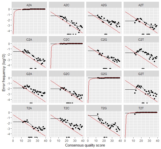
> plotErrors(errF, nominalQ=TRUE)

Hopefully you will see the image overleaf. So, what does this show? The error rates for each possible transition (e.g. A->C, A->G, …) are shown as “A2C”, “A2G” etc.. The points are the observed error rates (y-axis) for each consensus quality score (x-axis). The black line shows the estimated error rates after convergence. The red line is the error rates expected under the nominal definition of the Q-value. Here the black line (the estimated rates) fits the observed rates well, and the error rates drop with increased quality as expected. The tutorial states that everything looks reasonable and we proceed.

Question 6: How would you modify the previous code to draw a plot of the error estimations for the reverse reads?

____________________

Exercise 7: Sample inference

We are now ready to apply the core sequence-variant inference algorithm to the dereplicated data. What does that mean? Well, looking at the help for dada() - ?dada - indicates that “The dada function takes as input dereplicated amplicon sequencing reads and returns the inferred composition of the sample (or samples). Put another way, dada() removes all sequencing errors to reveal the members of the sequenced community.”

Let’s run this on the dereplicated forward and reverse reads (derepFs and derepRs) separately again, and then look at an example output for one sample:

### Infer the sequence variants in each sample
> dadaFs <- dada(derepFs, err=errF, multithread=TRUE)
Sample 1 - 7113 reads in 1979 unique sequences.
Sample 2 - 5299 reads in 1639 unique sequences.
Sample 3 - 5463 reads in 1477 unique sequences.
......

> dadaRs <- dada(derepRs, err=errR, multithread=TRUE)
Sample 1 - 7113 reads in 1660 unique sequences.
Sample 2 - 5299 reads in 1349 unique sequences.
Sample 3 - 5463 reads in 1335 unique sequences.
......

### inspect the results in more detail
> dadaFs[[1]]
dada-class: object describing DADA2 denoising results
128 sample sequences were inferred from 1979 input unique sequences.
Key parameters: OMEGA_A = 1e-40, OMEGA_C = 1e-40, BAND_SIZE = 16

Question 7: Using the last line of code above, adapt it to find out how many sample sequences were inferred for sample 15?

____________________

Exercise 8: Merging the paired reads

Now we can actually go ahead and merge our forward and reverse reads into a single read that overlaps. By doing this, we can also further reduce spurious sequence variants by merging these overlapping reads. The core function here is mergePairs(), which depends on the forward and reverse reads being in matching order at the time they were dereplicated.

### Merge the denoised forward and reverse reads
> mergers <- mergePairs(dadaFs, derepFs, dadaRs, derepRs, verbose=TRUE)
6540 paired-reads (in 107 unique pairings) successfully merged out of 6891 (in 197 pairings) input.
5028 paired-reads (in 101 unique pairings) successfully merged out of 5190 (in 157 pairings) input.
4986 paired-reads (in 81 unique pairings) successfully merged out of 5267 (in 166 pairings) input.
......

The resulting dataframe – called mergers – is large, so we will just look at the start of sample 1:

### Inspect the merger data.frame from the first sample
> head(mergers[[1]])
sequence
1 TACGGAGGATGCGAGCGTTATCCGGATTTATTGGGTTTAAAGGGTGCGCAGGCGGAAGATCAAGTCAGCGGTAAAATTGAGAGGCTCAACCTCTTCGAGCCGTTGAAACTGGTTTTCTTGAGTGAGCGAGAAGTATGCGGAATGCGTGGTGTAGCGGTGAAATGCATAGATATCACGCAGAACTCCGATTGCGAAGGCAGCATACCGGCGCTCAACTGACGCTCATGCACGAAAGTGTGGGTATCGAACAGG
2 TACGGAGGATGCGAGCGTTATCCGGATTTATTGGGTTTAAAGGGTGCGTAGGCGGCCTGCCAAGTCAGCGGTAAAATTGCGGGGCTCAACCCCGTACAGCCGTTGAAACTGCCGGGCTCGAGTGGGCGAGAAGTATGCGGAATGCGTGGTGTAGCGGTGAAATGCATAGATATCACGCAGAACCCCGATTGCGAAGGCAGCATACCGGCGCCCTACTGACGCTGAGGCACGAAAGTGCGGGGATCAAACAGG
.......
  abundance forward reverse nmatch nmismatch nindel prefer accept
1       579       1       1    148         0      0      1   TRUE
2       470       2       2    148         0      0      2   TRUE
3       449       3       4    148         0      0      1   TRUE
4       430       4       3    148         0      0      2   TRUE
5       345       5       6    148         0      0      1   TRUE
6       282       6       5    148         0      0      2   TRUE

Exercise 9: Constructing the sequence table and removing chimaeras

We can now construct a sequence table of our samples that is analogous to the “OTU table” produced by classical methods. We do not want to run this on the mock community samples as we are using those at the end of the practical, if there is time.

### Construct sequence table of the non-Mock data
> seqtab <- makeSequenceTable(mergers)

The sequence table – seqtab – is a matrix with rows corresponding to (and named by) the samples, and columns corresponding to (and named by) the sequence variants.

Question 8 Use the dim() function to find out the size of seqtab.

____________________

We can now look at the distribution of the sequence lengths:

### Inspect the distribution of sequence lengths
> table(nchar(getSequences(seqtab)))

Question 9 What is the most frequent size for seqtab?

____________________

Our merged sequences all fall in the expected range for the V4 amplicon as described by the Illumina protocol, so this is reassuring.

The core dada() method removes substitution and indel errors, but chimaeras remain. Fortunately, the accuracy of the sequences after this denoising process makes identifying chimaeras easier than it is when dealing with fuzzy OTUs: all sequences which can be exactly reconstructed as a bimera (two-parent chimera) from more abundant sequences. Let’s see what happens when we remove chimaeras:

### Remove chimeric sequences 
> seqtab.nochim <- removeBimeraDenovo(seqtab, verbose=TRUE)
Identified 61 bimeras out of 293 input sequences.

Question 10 Use the dim() function to find out the size of seqtab.nochim?

____________________

This is not the same as sebtab. Let’s calculate our sequences remaining after checking for chimaeras:

> sum(seqtab.nochim)/sum(seqtab)
[1] 0.9640374

The fraction of chimeras varies based on factors including experimental procedures and sample complexity but can be substantial. Here chimeras make up about 21% of the inferred sequence variants (61 out of 293), but those variants account for only about 4% of the total sequence reads.

Exercise 10: Checking our progress

We can do a quick check of how our samples have performed over the process to get to this stage. This is important as it can be regarded as a “sanity check” before we went on and did more analyses if we so wished. If we saw an over-large drop associated with one step, we might want to have a look at our parameters throughout our sequence processing.

### Remove chimeric sequences with some complicated code 
> getN <- function(x) sum(getUniques(x)) # our first function
> track <- cbind(trim_data, sapply(dadaFs, getN), sapply(dadaRs, getN),
           sapply(mergers, getN), rowSums(seqtab.nochim))

> colnames(track) <- c("input", "filtered", "denoisedF", "denoisedR", "merged",
                       "nonchim")
                       
> rownames(track) <- sample.names

> head(track)
       input filtered denoisedF denoisedR merged nonchim
F3D0    7793     7113      6976      6979   6540    6528
F3D1    5869     5299      5227      5239   5028    5017
F3D141  5958     5463      5331      5357   4986    4863
F3D142  3183     2914      2799      2830   2595    2521
F3D143  3178     2941      2822      2868   2553    2519
F3D144  4827     4312      4151      4228   3646    3507

Exercise 11: Assigning taxonomy

So, here we are at last, at the point, after having done all this quality control work, of actually looking at what all these sequences mean, as far as a taxonomic classification is concerned. It is common at this point in 16S/18S/ITS amplicon sequencing, to classify sequence variants taxonomically.

The DADA2 package provides a native implementation of the RDP’s naive Bayesian classifier for this purpose. The assignTaxonomy() function takes a set of sequences and a training set of taxonomically classified sequences, and outputs the taxonomic assignments with at least minBoot bootstrap confidence. Again, this step might take three minutes or so, so please be patient. We will use a small reference dataset to classify the seqtab.nochim sequences to, and then use the taxa.print() function to remove the names and print them out:

### use a reference data set to assign taxonomy to the reads
> training <- ("/cloud/project/silva_nr_v132_train_set.fa.gz")
> training
[1] "/cloud/project/silva_nr_v132_train_set.fa.gz"

> taxa <- assignTaxonomy(seqtab.nochim, training, multithread=TRUE)

### Removing sequence rownames for display only
> taxa.print <- taxa 
> rownames(taxa.print) <- NULL
> head(taxa.print)
     Kingdom    Phylum          Class         Order           Family           Genus        
[1,] "Bacteria" "Bacteroidetes" "Bacteroidia" "Bacteroidales" "Muribaculaceae" NA           
[2,] "Bacteria" "Bacteroidetes" "Bacteroidia" "Bacteroidales" "Muribaculaceae" NA           
[3,] "Bacteria" "Bacteroidetes" "Bacteroidia" "Bacteroidales" "Muribaculaceae" NA           
[4,] "Bacteria" "Bacteroidetes" "Bacteroidia" "Bacteroidales" "Muribaculaceae" NA           
[5,] "Bacteria" "Bacteroidetes" "Bacteroidia" "Bacteroidales" "Bacteroidaceae" "Bacteroides"
[6,] "Bacteria" "Bacteroidetes" "Bacteroidia" "Bacteroidales" "Muribaculaceae" NA   

So, at this point we could stop, as we have a taxonomy, ready for phyloseq in Practical 9 in two week’s time for further analysis and visualisation. However, we can do one more thing today.

Exercise 12: Evaluating the accuracy

Our last thing to do with this dataset from a DADA2 point of view is to evaluate the accuracy in terms of how well the process has gone with these sequence data, and we can use a “mock community” for this purpose. This is a mixture of 20 known strains (this mock community is supposed to be 21 strains, but the bacterium P. acnes was absent). Reference sequences corresponding to these strains were provided in the downloaded zip archive. Previously, the Mock sample was removed when we made the sequence table, but we return to that sample now and compare the sequence variants inferred by DADA2 to the expected composition of the community.

### Evaluating DADA2’s accuracy on the mock community
> unqs.mock <- getUniques(removeBimeraDenovo(mergers[["Mock"]], verbose=TRUE))
Identified 0 bimeras out of 20 input sequences.

### how did we do? – we are printing information out to the screen now in a different way
> cat("DADA2 inferred", length(unqs.mock), "sample sequences present in the Mock community.\n")
DADA2 inferred 20 sample sequences present in the Mock community.

### find our reference file – don’t worry about this complex code
> mockRef <- readFasta(file.path(path, "HMP_MOCK.v35.fasta"))
> match.ref <- sum(sapply(names(unqs.mock), function(x) any(grepl(x, as.character(sread(mockRef))))))

### print out our results
> cat("Of those,", sum(match.ref), "were exact matches to the expected reference sequences.\n")
Of those, 20 were exact matches to the expected reference sequences.

This mock community dataset contained 20 bacterial strains. DADA2 found 20 unique sequences all of which exactly match the reference genomes of the expected community members. The residual error rate after the DADA2 pipeline for this sample is 0%. In comparison, the tutorial records that the mothur pipeline finds 34 OTUs in this Mock community sample. DADA2 infers sequence variants exactly instead of fuzzy 97% OTUs, and outputs fewer false positives than the OTU methods!

We are now at the end of the DADA2 tutorial, and further work will be picked up again in Week 9. However to complete today’s practical, we are going to do something else with our sequencing data.

Exercise 13: Working with fasta files to generate a sequence logo

I covered the theory around sequence logos in the Tuesday tutorial, but if you are interested in the maths behind this (information content and bits), the base information can be found on the Wikipedia sequence logo page.

We have created a dataframe of 232 16S rRNA sequences called seqtab.nochim that represent the sequences in our experiment. We now consider these sequences as unique sequences, even though we know that they are present at vastly different proportions in the 20 samples we have. However, we are going to ignore that fact for now and make a fasta file of these sequences for illustrating the principles required for the Portfolio Analysis. To do this, we need to load some pre-installed packages in order to create a fasta file that we can do further analysis on.

> library(FastaUtils)
> library(msa)
> library(seqLogo)
 
### make a fasta file from the nochim dataframe
> uniquesToFasta(seqtab.nochim, "nochimSeqs232.fa")

### make a random subsample of say 100 sequences
> fasta.sample(infile = "nochimSeqs232.fa", nseq = 100, file.out = "sub100_nochimSeqs.fa")

As we are randomly pulling sequences in this section, the output will look slightly different from one attempt to the other in the below.

To illustrate the path from fasta sequence file to aligned sequence to a sequence logo, we will use the fasta file sub100_nochimSeqs.fa as an example of the workflow.

### import the sequences to work with them
> seqs16S <- readDNAStringSet("sub100_nochimSeqs.fa")

### run the sequence alignment and view in the console
> my16SAlignment <- msa(seqs16S) 
use default substitution matrix

> my16SAlignment
CLUSTAL 2.1  

Call:
   msa(seqs16S)

MsaDNAMultipleAlignment with 100 rows and 258 columns
      aln                                                                                          names
  [1] GACAGAGGATGCAAGCGTTATCCGGAATGATTGGGCGTAAAGCGT...CGAC-ACTGACACTGAG-AGACGAAAGCTAGGGGAGCGAATGGG sq222;size=5;
  [2] GACAGAGGATGCAAGCGTTATCCGGAATGATTGGGCGTAAAGCGT...CGAC-ACTGACACTGAG-AGACGAAAGCTAGGGGAGCGAATGGG sq189;size=18;
....

[100] GACGGGGGGGGCAAGTGTTCTTCGGAATGACTGGGCGTAAAGGGC...CCCT-ACCGACGCTGGG-GTGCGAAAGCATGGGGAGCGAACAGG sq107;size=117;
  Con TACGTAGGGGGCAAGCGTTATCCGGATTTACTGGGTGTAAAGGGA...?GTA-ACTGACGCTGAG-GCTCGAAAGCGTGGGGAGCAAACAGG Consensus
  
> print(my16SAlignment, show="complete") # view the results

MsaDNAMultipleAlignment with 100 rows and 258 columns
      aln (1..92)                                                                                  names
  [1] GACAGAGGATGCAAGCGTTATCCGGAATGATTGGGCGTAAAGCGT-CTGTAGGTGGCTTTTTAAGTCCGCCGTCAAAT-CCCAGGGCTCAAC sq222;size=5;
  [2] GACAGAGGATGCAAGCGTTATCCGGAATGATTGGGCGTAAAGCGT-CTGTAGGTGGCTTTTTAAGTTCGCCGTCAAAT-CCCAGGGCTCAAC sq189;size=18;

.....

 [99] AACACCGGTGGCGAAGGCGGGTCTCTGGGCCGTT-ACTGACGCTGAG-GAGCGAAAGCGTGGGGAGCGAACAGG sq58;size=325;
[100] AACGCCAAAAGCGAAGGCAGCTCTCTGGGTCCCT-ACCGACGCTGGG-GTGCGAAAGCATGGGGAGCGAACAGG sq107;size=117;
  Con AACACCAGTGGCGAAGGCGGCTT?CTGGAC?GTA-ACTGACGCTGAG-GCTCGAAAGCGTGGGGAGCAAACAGG Consensus 

### print out the alignment
> msaPrettyPrint(my16SAlignment, output="pdf", showNames="left", file = "ourSet.pdf",
                showLogo="top", askForOverwrite=FALSE, verbose=FALSE)

The msaPrettyPrint() command has lots of options including showing the sequence names and printing out certain regions only. I would strongly suggest giving ?msaPrettyPrint a look and to understand what is going on.

We can also use the seqLogo package to generate a sequence logo only. This package has limited functionality and printing ability and is probably designed for shorter sequence stretches, as discussed in the tutorial. The code is a little complex, so it has comments for each code section. Please do not worry too much about what the code is doing here.

### generate a sequence logo only using the seqLogo package

## read in only the first 150 positions in the alignment
> smallAlign <- DNAStringSet(my16SAlignment, start=1, end=150)

## use seqLogo to make a consensus matrix
> posWeightMat <- consensusMatrix(smallAlign, baseOnly=TRUE)

## remove the 'other' row to give only A, C, G and T counts
> rowname_to_remove <- ("other")
> posWeightMat2 <- posWeightMat[!(row.names(posWeightMat) %in% rowname_to_remove),]

## proportionate per alignment position
> posWeightMat2 <- prop.table(posWeightMat2, 2)
> p <- makePWM(posWeightMat2)

## print out the logo with a smaller font size than usual
> seqLogo(p, xfontsize = 10)

You could then export this image to save it through the Export command in the Plots view in the bottom right window.

Portfolio analysis

There are two parts to the week 8 Portfolio analysis. This will result in a figure with a part A and a part B.

Part A

From Exercise 10, you generated a dataframe called track with dimensions of 6 columns and 20 rows.

Your task is to plot this dataframe in a way that shows whether the multiple steps in the processing are adversely affecting (or not) one or more samples. Consider the dataframe from left to right, as there is a general reduction in the number of sequences at each stage from left to right. The columns ‘denoisedF’ and ‘denoisedR’ are a little different, but leave them as they are. Remember to get inspiration and ideas from https://r-graph-gallery.com/. Would you plot the data as is, would you proportionate, and if so, by rows or columns? If this was a way to go, as a hint, the function prop.table() could be of use, as was used for a different purpose in Exercise 13 above.

Part B

From Exercise 13, you worked with a method to generate a sequence logo from the sequences from the DADA2 tutorial. Unfortunately, due to its scale, this is not a dataset with a lot of sequence variation within it. To get to looking at a truer represenation of the 9 hypervariable regions within 16S rRNA, we need to use a reference fasta file such as rdp_train_set_14.fa.

Your task is to generate a new fasta file of 50 sequences chosen at random, and search with the msa and seqLogo packages to find a region of ~100 - 150 bp in length that shows a high degree of sequence similarity and then variability. You should then also plot the same region with the msa package showing the alignment and the sequence logo, describing what you observe in the figure legend.

Guiding thoughts for the portfolio

Part A

Things to consider for plotting:

i) Even though track is a dataframe, do you want to keep it like that? Would it help if was of a different data class?

> class(track)
[1] "data.frame"

What about converting it to a data matrix (Goolging will find an answer to this quickly) to give more flexibility? Please remember the difference between dataframes and data matrices. A data matrix allows you to consider other plotting functions such as:

-> Barplots

-> Heatmaps

-> Stacked barplot

ii) Now you have decided on a visualisation method, do you plot the data as raw data – the numbers you have already in track – or do you transform them somehow? I mentioned prop.table() above as a potential function to use. Have a look at the help with:

> ?prop.table

to see what the code is for proportioning on rows or columns.

iii) Please note that some of the guiding code at https://r-graph-gallery.com/ uses the ggplot2 library. Whilst we have not taught this explicitly in the course, there are methods out there on such pages that hopefully you will be able to adapt for your situation.

iv) It’s a good idea to save your portfolio code and to maybe to start off with a copy of the track object and work with that, so your original version is not damaged:

> trackCopy <- track
> dim(track)
[1] 20  6
> dim(trackCopy)
[1] 20  6

Part B

i) First of all, there is no perfect region here, there are many regions to choose from across the alignment, and as you are making a random subset, in theory everyone’s alignment will be subtly different.

ii) The reference fasta file we are using – rdp_train_set_14.fa – has a great range of sequence length within it. For your information (i.e. there is no need to do this):

/cloud/project$ seqkit stats rdp_train_set_14.fa
file                 format  type  num_seqs     sum_len  min_len  avg_len  max_len
rdp_train_set_14.fa  FASTA   DNA     10,678  15,409,307      320  1,443.1    2,210

so as you can see, a wide range. This will result in a large alignment visualised with msaPrettyPrint(). In orer to find an area of interest as above with the way the printing works, look at the options with msaPrettyPrint() to find a way to remove the names temporaily as this will maximise the alignment in the PDF, and there are less pages to visually inspect.

iii) Choosing the ~100 - 150bp region is up to you. Once you have a region, I would suggest getting that smaller region clarified with msa (as a new object maybe), and then using the same region coordinates (i.e., start and end) for visualising the alignment with seqLogo.

Assessment

To reiterate, there is no direct assessment today. What is required however, is an understanding of the principles we have learnt today, as these will be required for the mastery test which accounts for 15% of the course. This will take place between Thursday 25-May-2023 and Friday 26-May-2023 online.

The mastery test will test the contents of weeks 8 to 10, more information will follow soon.

Contact

I have two offices on the Manawatu campus (as I work for both SNS and SoVS), so I am not always in my Science Tower office D5-30. If you want to discuss anything, it’s best to email me beforehand.

Prof Patrick Biggs,

Molecular Biosciences Group,

School of Natural Sciences

-. .-.   .-. .-.   .-. .-.   .
||\|||\ /|||\|||\ /|||\|||\ /|
|/ \|||\|||/ \|||\|||/ \|||\||
~   `-~ `-`   `-~ `-`   `-~ `-

p.biggs@massey.ac.nz

Callahan et al. Nature Methods 13:581–583. (2016) ↩
Concepts for this part of the practical came from a tutorial found at: https://benjjneb.github.io/dada2/tutorial.html ↩

Genome Science 203.311

Genome Science for Genome Scientists

Barcodes and diversity - Fastq read analysis for 16S rRNA metabarcoding using the R package DADA2

Purpose

Introduction

Lecture Overview

Conventions used for this RStudio practical

Accessing the resources needed

Computing

General

Manawatu (iMacs)

Albany (PCs)

outside Massey

Our work today

Theoretical overview

What we are going to do today?

Exercise 1: Getting everything ready

Exercise 2: Collecting our data

Exercise 3: Examining the quality profiles of forward and reverse reads

Exercise 4: Performing filtering and trimming

Exercise 5: Dereplication

Exercise 6: Investigation of the error rates

Exercise 7: Sample inference

Exercise 8: Merging the paired reads

Exercise 9: Constructing the sequence table and removing chimaeras

Exercise 10: Checking our progress

Exercise 11: Assigning taxonomy

Exercise 12: Evaluating the accuracy

Exercise 13: Working with fasta files to generate a sequence logo

Portfolio analysis

Part A

Part B

Guiding thoughts for the portfolio

Part A

Part B

Assessment

Contact